Examples
There is no better way to get familiar with pylion than to dive straight into a couple of example scripts.
There are more scripts in the examples folder.
Also, you might find a lot of the tests useful since most of them test physics.
Simple example
This is as simple as it gets. Within a few lines of code, we setup a setup a simulation that outputs the trajectories and veolcities of 100 atoms in a linear Paul trap:
import pylion as pl

s = pl.Simulation('simple')

ions = {'mass': 40, 'charge': -1}
s.append(pl.createioncloud(ions, 1e-3, 100))

trap = {'radius': 3.75e-3, 'length': 2.75e-3, 'kappa': 0.244,
        'frequency': 3.85e6, 'voltage': 500, 'endcapvoltage': 15}
s.append(pl.linearpaultrap(trap))

s.append(pl.langevinbath(0, 1e-5))

s.append(pl.dump('positions.txt', variables=['x', 'y', 'z'], steps=10))
vavg = pl.timeaverage(20, variables=['vx', 'vy', 'vz'])
s.append(pl.dump('secv.txt', vavg, steps=200))

s.append(pl.evolve(1e4))
s.execute()
First, import pylion and instantiate a Simulation() object.
Using the functions createioncloud() and linearpaultrap() we generate a cloud of 100 ions and a trap with the given parameters and append them to the simulation.
The ions are in contact with a langevin bath that damps their motion.
We evolve the ensemble for 1e4 steps, outputing the position of each ion every 10 steps and the velocity average every 200 steps which corresponds to one rf cycle.
Energy minimisation in a pseudopotential
This example first finds the positions of the ions that correspond to the minimum energy of the system. After that it evolves the atoms using the full rf potential and plots the output. Here’s the whole script:
import pylion as pl
from pathlib import Path
import matplotlib.pyplot as plt
from mpl_toolkits.mplot3d import Axes3D

# use filename for simulation name
name = Path(__file__).stem

s = pl.Simulation(name)

ions = {'mass': 30, 'charge': -1}
s.append(pl.createioncloud(ions, 1e-3, 10))

trap = {'radius': 7e-3, 'length': 5.5e-3, 'kappa': 0.244,
        'frequency': 3.85e6, 'voltage': 300,
        'endcapvoltage': -0.01, 'pseudo': True}
pseudotrap = pl.linearpaultrap(trap, ions)
s.append(pseudotrap)

s.append(pl.minimise(0, 0, 10000, 10000, 1e-7))
s.remove(pseudotrap)

trap['pseudo'] = False
s.append(pl.linearpaultrap(trap))

s.append(pl.langevinbath(3e-4, 1e-5))
s.append(pl.thermalvelocities(3e-4))

s.append(pl.dump('positions.txt', variables=['x', 'y', 'z'], steps=100))

s.append(pl.evolve(1e4))

s.execute()

_, data = pl.readdump('positions.txt')
data *= 1e6

fig = plt.figure()
ax = fig.add_subplot(111, projection='3d')
ax.scatter(data[10:-10:10, :, 0], data[10:-10:10, :, 1], data[10:-10:10, :, 2])
ax.scatter(data[-1, :, 0], data[-1, :, 1], data[-1, :, 2],
           c='red', s=50, alpha=1)
ax.scatter(data[0, :, 0], data[0, :, 1], data[0, :, 2],
           c='blue', s=50, alpha=1)
plt.xlabel('x (um)')
plt.ylabel('y (um)')
plt.zlabel('z (um)')
plt.show()
First, import pylion and a few other packages.
Then you will need to instantiate a Simulation object that takes name as its single parameter.
It’s not a bad idea to use the name of the file for that.
The simulation parameters are largely contained in two dictionaries, ions and trap.
Here, we use createioncloud() to generate a cloud of 10 ions randomly positioned within a sphere with radius 1mm, and append them to the simulation.
Similarly we define a Paul trap using linearpaultrap().
We then call minimise() to get the groundstate configuration of the atomic cloud which for these parameters is a linear ion chain.
After the minimisation we remove the pseudopotential trap, and append another trap with the same parameters but with the full rf potential.
The ions at this stage have thermal velocities defined by thermalvelocities() and are in contact with a langevin bath so their motion is damped.
We let the simulation evolve for 1e4 steps, dumping the positions of the ions to the file positions.txt every 100 steps.
The Simulation object validates its input as it is appended but nothing happends till we call execute().
A lammps subprocess begins here, which should only take a few moments after which we can read in the data and plot it.
Rigid bodies
In this example we define a group of ions to be rigidly connected and act like a one-dimensional charged rod:
import pylion as pl
from pathlib import Path
import matplotlib.pyplot as plt
from mpl_toolkits.mplot3d import Axes3D
import matplotlib.animation as animation

# use filename for simulation name
# name = Path(__file__).stem

s = pl.Simulation(name)

ions = {'mass': 40, 'charge': 1}
s.append(pl.createioncloud(ions, 1e-3, 50))

rod = {'mass': 40, 'charge': 1, 'rigid': True}
positions = [[1e-4, -0.5e-5, 0], [1e-4, 0, 0], [1e-4, 0.5e-5, 0]]
s.append(pl.placeions(rod, positions))

trap = {'radius': 3.75e-3, 'length': 2.75e-3, 'kappa': 0.244,
        'frequency': 3.85e6, 'voltage': 500, 'endcapvoltage': 15}
s.append(pl.linearpaultrap(trap))

s.append(pl.langevinbath(0, 1e-5))

s.append(pl.evolve(1e4))

s.append(pl.dump('positions.txt', variables=['x', 'y', 'z'], steps=2))
vavg = pl.timeaverage(20, variables=['vx', 'vy', 'vz'])
s.append(pl.dump('secv.txt', vavg, steps=20))

s.append(pl.evolve(1000))
s._writeinputfile()
s.execute()

_, data = pl.readdump('positions.txt')
data *= 1e6

fig = plt.figure()
ax = fig.add_subplot(111, projection='3d')
p1 = ax.scatter(data[0, :50, 0], data[0, :50, 1], data[0, :50, 2], alpha=0.8)
p2 = ax.scatter(data[0, -3:, 0], data[0, -3:, 1], data[0, -3:, 2],
                c='r', s=80, alpha=0.8)
ax.set_xlim([-60, 60])
ax.set_ylim([-60, 60])
ax.set_zlim([-60, 60])
ax.set_xlabel('x $(\mu m)$')
ax.set_ylabel('y $(\mu m)$')
ax.set_zlabel('z $(\mu m)$')
# plt.show()


# 3D animation
def update_points(frame):
    p1.set_offsets(frame[:50, :2])
    p1.set_3d_properties(frame[:50, 2], 'z')
    p2.set_offsets(frame[-3:, :2])
    p2.set_3d_properties(frame[-3:, 2], 'z')


anim = animation.FuncAnimation(fig, update_points, frames=data,
                               interval=20, repeat=True)
# anim.save('anim.mp4', fps=10)  # ffmpeg needs to be installed
plt.show()
The declarations should feel generally familiar by now except for the ion placement syntax.
The ions dictionary has the additional keyword rigid set to true and we use placeions() to place the ions by hand so that we define the geometry of the rod.
After executing the simulation, you can see an animation of the charged rod and the other ions in the cloud oscillating in the trap.
Secular resonances of a single ion in a spherical Paul trap
Here we compare secular resonances from simulated single ion trajectories in an endcappaultrap() to the low-order and
high-order approximations in Lindvall2022 “High-Accuracy Determination of Paul-Trap Stability Parameters for
Electric-Quadrupole-Shift Prediction”.
The trap and ion definitions used are:
trap = {'z0': 0.86e-3/2,  'frequency': 14.424e6,
       'voltageRF': 300.0, 'etaRF': 0.97, 'eps':5e-2,
       'voltageDC': 0.0, 'etaDC': 0.97, }
ions = {'mass': 88, 'charge': 1} # a single Strontium ion
where voltageRF was varied between 100 V and 300 V. Ion trajectories were simulated for 10e6 timesteps of 0.25 ns each,
for a total simulation time of 2.5 ms. This corresponds to
around 1000 oscillations at the lowest secular frequencies (ca 400 kHz).
The three secular resonances (two radial modes X and Y, split due to trap asymmetry eps, and one axial mode Z) were
determined from ion position trajectories by computing the power spectral density (PSD) with scipy.signal.welch and fitting
a Lorentzian to the PSD with scipy.optimize.curve_fit. Results were compared to the low-order (\(\beta_{i,LO}\)) and
high-order (\(\beta_{i,HO}\)) approximations
provided by the endcap_secular() function
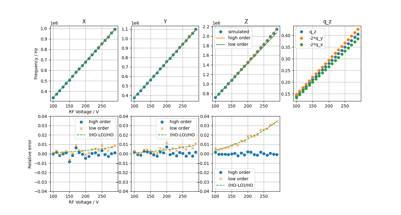
The results show that the high-order approximation agrees with simulation to better than 1%, while the low-order approximation deviates from simulated results by up to 4% at high trap drive voltages.
Excess micromotion of a single ion in a spherical Paul trap
When determining the differential static scalar polarizability (DSSP) for ions with a negative DSSP using the magic-RF frequency method (Dube2014, Huang2019, Lindvall2025), knowing the relative strength of the oscillating electric field at harmonics of the trap drive frequency \(\Omega\) seen by the ion (or the ion velocity) is essential.
Dube2014, Huang2019 used an approximation to second order in \(\Omega\):
while a third-order solution is used in Lindvall2025: